Autonomous Line Follower

Grand PrIEEE 2017

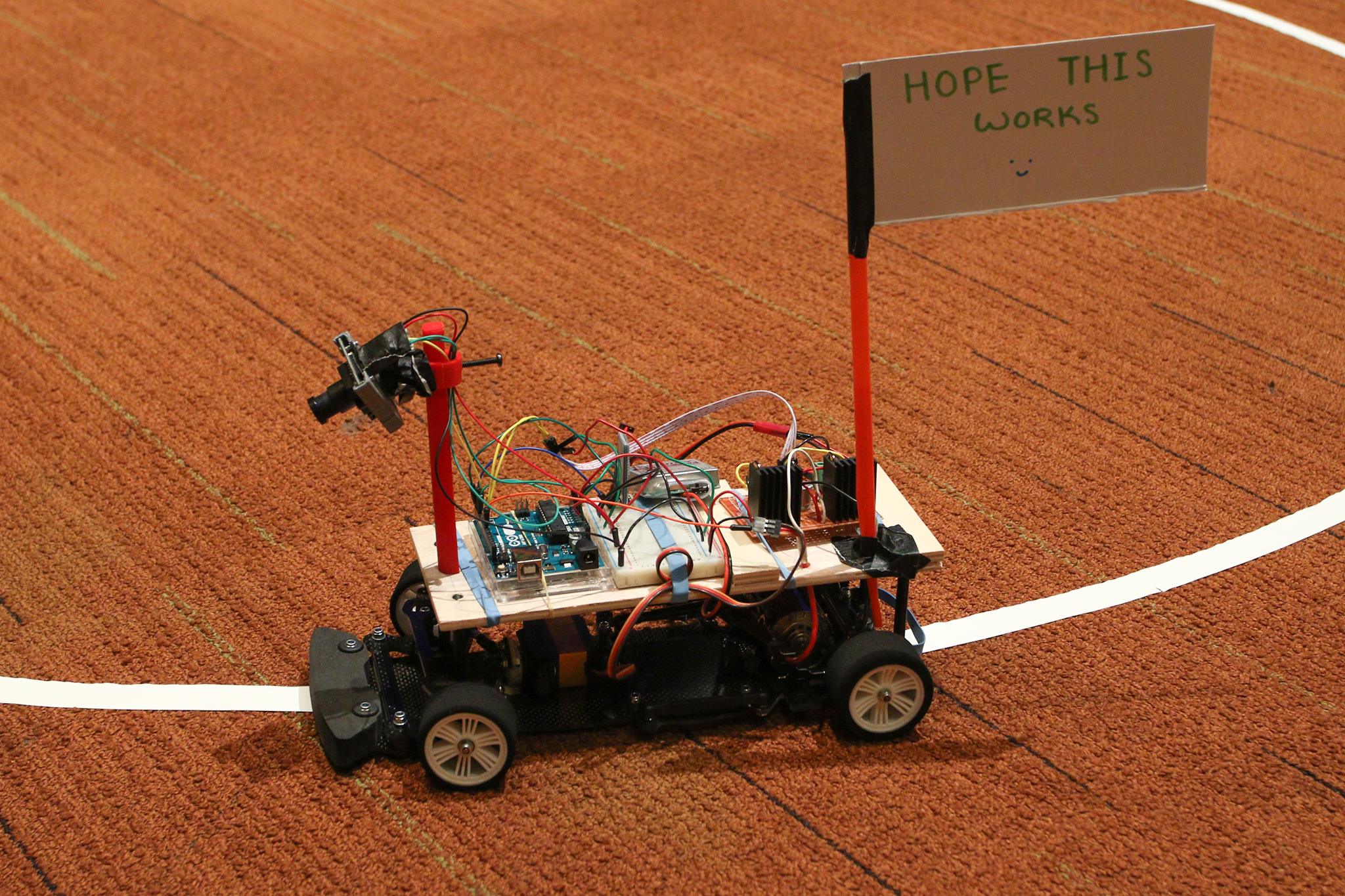
During the 2016-2017 school year, I worked on a project called Grand PrIEEE. It is a yearlong project where multiple teams create a small autonomous vehicle that would navigate through a preset track made of white tape. At the end of the year, the teams would compete against each other for the quickest completion time. This competition was hosted by UCSD’s IEEE club.

In my group, I worked with 3 other people. My contributions include: selecting hardware/vehicle components, completing the H bridge motor driver circuit, assembling the system, and working on the overall line detection code.

System Architecture

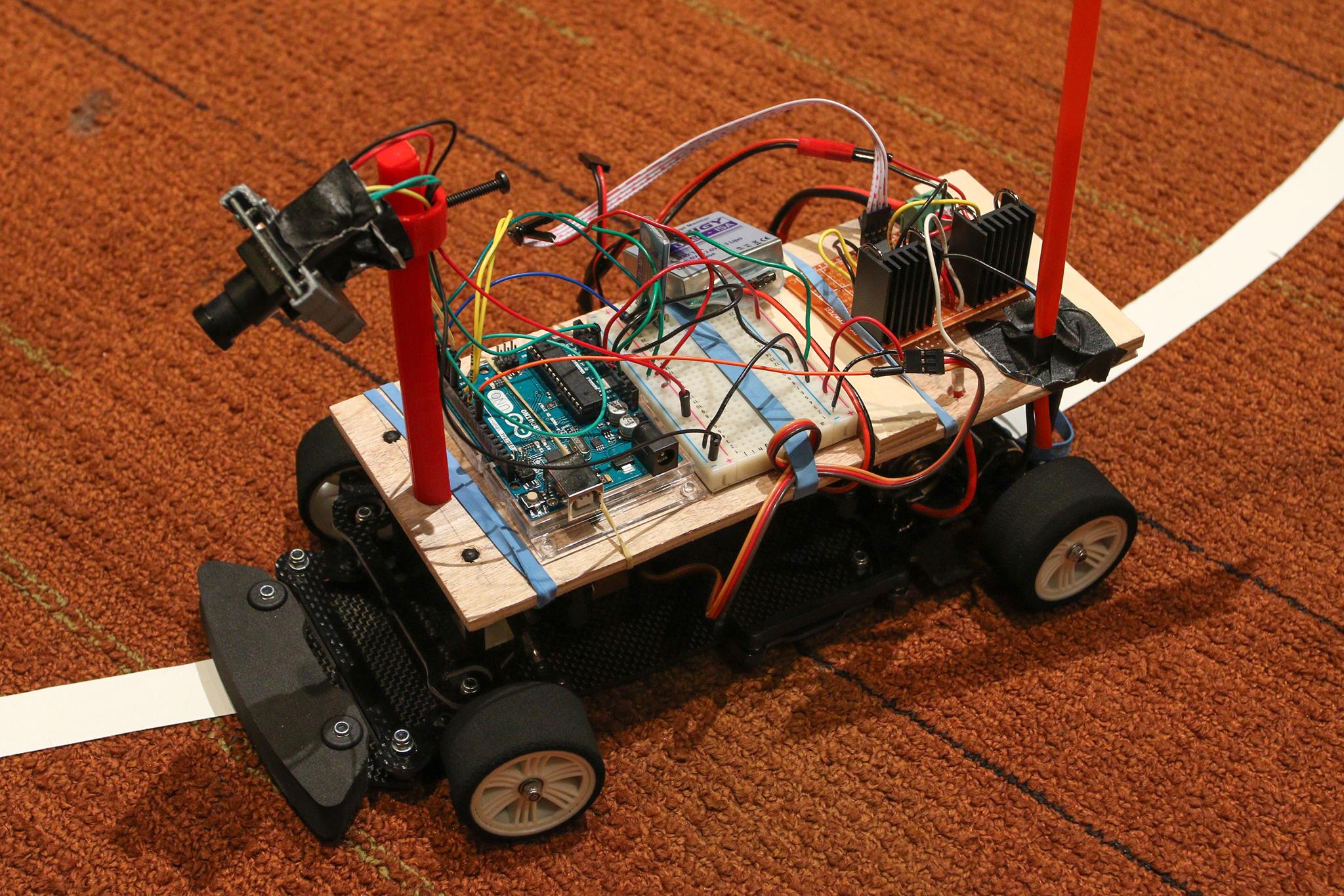
Here are our main components:
Arduino Uno
Schumacher Supastox GT 1/12 Scale Chassis
Fluoreon 3S 11.1V 1500 mAh LiPo Battery
Savox SC-1258TGT Digital Servo
HC-06 Bluetooth Module
Parallax TSL1401 Linescan Camera
6v/5v UBEC Voltage Regulator

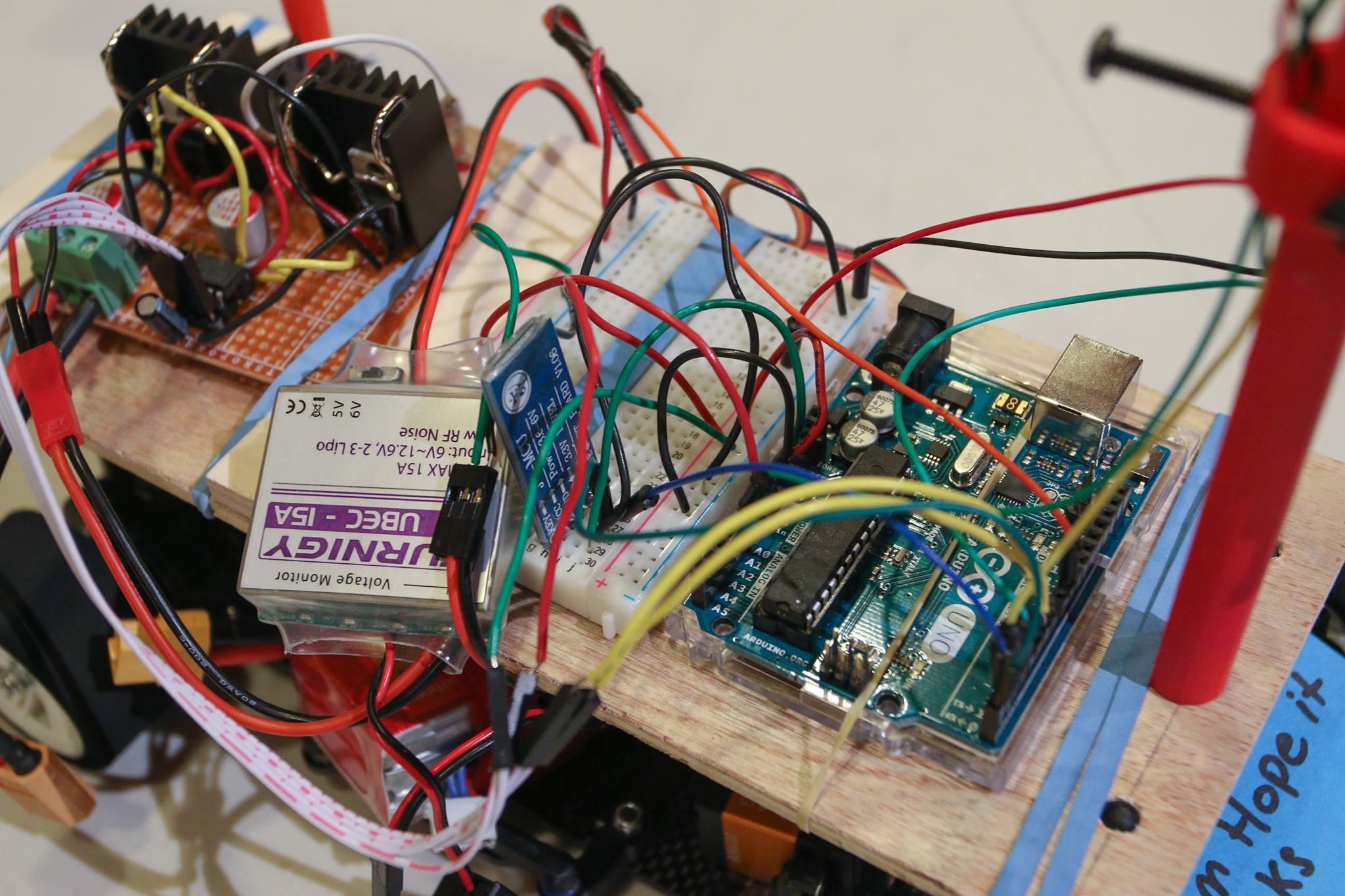
Our hardware system operated as follows:
A 12 volt LiPo battery was connected to the half bridge motor driver circuit.
The 12 volt driver powered and controlled the speed of the motor.
The 12 volt battery was also connected to a UBEC (Universal Battery Elimination Circuit), which regulated a 6 volt output. This 6 volt output powered the Arduino and steering servo.
The Arduino’s 5 volt pins were used to power the bluetooth module and linescan camera.

Our software system operated as follows:
The Arduino sent a PWM signal to the motor driver circuit such that the motor ran at a constant speed.
The Arduino would continuously read data from the linescan camera so determine the location of the white line track.
The steering servo was shifted accordingly to our proportional controller code so that the car stays on track.
The motor could be shut off remotely via cellphone app by issuing commands to the bluetooth module.

Half Bridge - Component Selection

For the motor, our project advisor suggested that our motor should have a minimum of 20 turns. Turns refers to the number of coil windings in brushed motors. Generally, more windings correspond to higher torque but less speed. We opted for the 27T brushed motor due to price, torque, and compatibility with our chassis.

The manufacturer’s data sheet specified a voltage range between 2.4V and 30V. It has a rated 5.02 Amp current draw at 7.2V. However, the data sheet does not mention stall current at all. We did managed to find some similar motors that had stall currents of around 50 amps. The stall current refers to the current draw when the motor shaft cannot physically turn anymore. Although it is unlikely, the motor can stall in our application if the car crashes into a wall or if the wheel becomes stuck somehow. Therefore, we needed to design a driver circuit that would supply up to 50 amps so that our circuitry wouldn’t burn out in an emergency.

Since the car only needs to go forward and not reverse, we opted for a half bridge driver instead of a full bridge. To design the circuit, I chose the switching MOSFETS based on the previous motor specifications. Component websites, such as DigiKey, had a huge selection of MOSFETs with varying specifications, so it was difficult to narrow down one. In the end, I opted for the FDP070AN06A0 because it had ratings that suited our application.

The datasheet shows that this NMOS is rated for 80 Amps at 10 volts, meaning that it could provide enough current if the motor were to stall. It also has a maximum voltage rating of 60 volts, so our 11.1 volt LiPo battery would work fine. Additionally, this NMOS has a low ‘Rds(on)’ and low input capacitance when compared to other MOSFETs. Rds(on) corresponds to the resistance between drain and source when the MOSFET is switched on. A lower resistance value is optimal because it would result in less power dissipation and less heat.

Input capacitance refers to the capacitance between the gate and source. For the NMOS to be fully switched on, the voltage between gate and source needs to be above a certain threshold. But before this voltage is “applied”, the gate capacitance has to be completely discharged. Thus, a lower gate capacitance is optimal because it results in faster switching between cut-off and saturation modes. This corresponds to less time wasted in triode mode (which has high heat dissipation).

Half Bridge - Initial Circuit Design

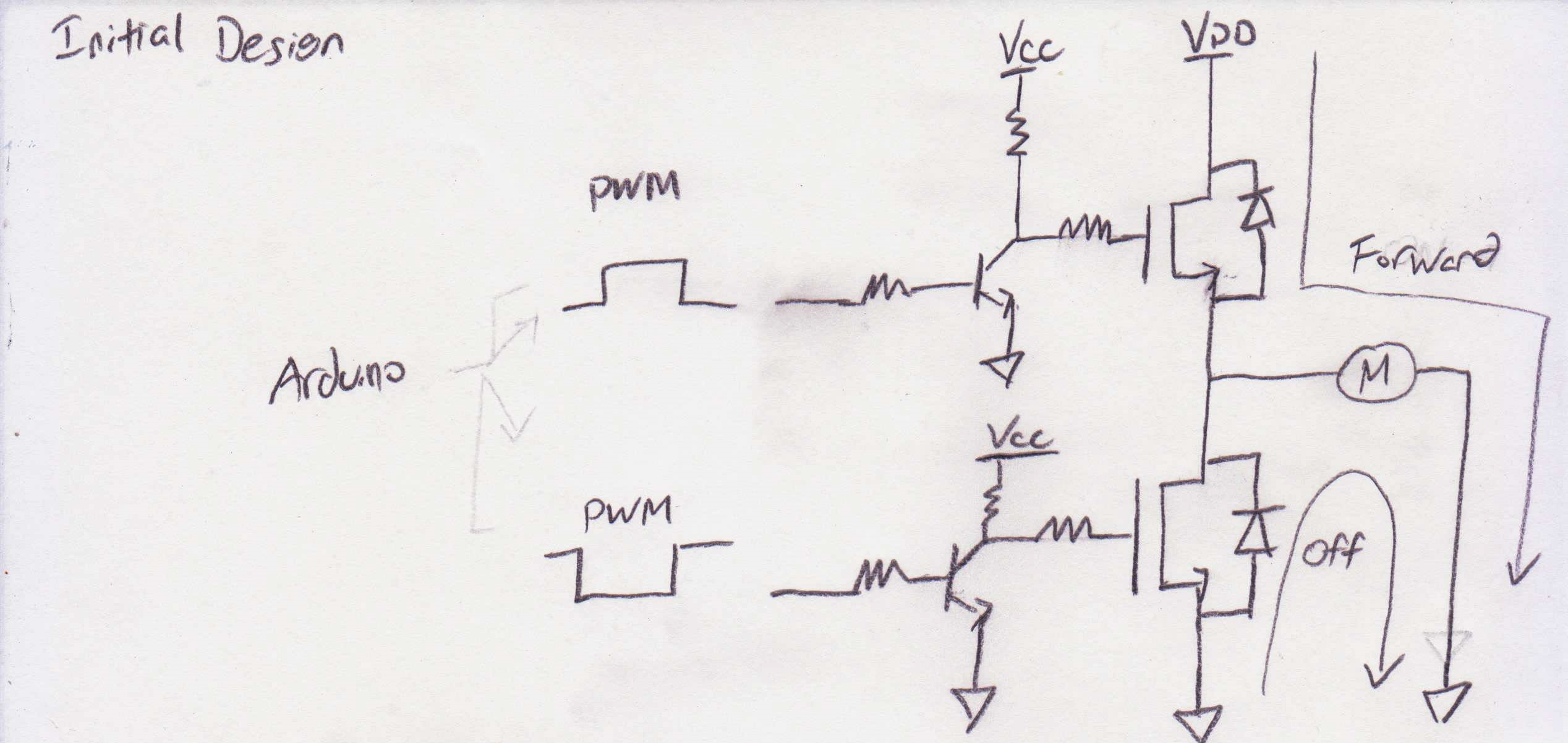
The sketch above depicts our early design for the half bridge circuitry. We would have a high side and low side MOSFET, each connected to a NPN BJT. The BJTs would serve as switches that would turn the MOSFETs on or off. The BJTs themselves would be biased by PWM pulses from the Arduino. The duty cycle of the PWM pulses would then dictate the speed of the motor. The pulses for the high side and low side drivers would be inverted out of phase such that only one side could be active high at any time.

When the high side is on and low side is off, current would flow through the motor and power the motor.
When the high side is off and low side is on, the motor would be grounded and turned off. Diodes would be place in parallel to the MOSFETs so that flyback currents from the motor startup wouldn’t damage the circuitry.

Half Bridge - Initial Design Drawbacks

Our initial design had some drawbacks. For instance, the PWM pulses from the Arduino are not very accurate, so the high side and low side signals may not be completely out of phase. If both MOSFETs were to be switched on at the same time, then they would be shorted and burnt out in a smoky blaze. To combat this, we needed a “dead-time” in the pulses. The dead time refers to an interval in the PWM pulses where both signals would be off simultaneously. This dead time would occur before the signal switches from high/low and low/high so that they can’t be high at the same time.

Another drawback was that our initial design had a high side PMOS and low side NMOS. Compared to NMOS, a PMOS is disadvantageous because it has a higher resistance when switched on. Additionally, the PMOS has higher input capacitance and therefore takes a longer time to switch between states. Therefore, we sought to use NMOS for both the high side and low side drivers.

However, this configuration was harder to implement. For a NMOS to be active, its gate-source voltage has to be above an intrinsic threshold. In this case, the source of the high side NMOS is connect to the load. The voltage drop across the NMOS is minimal, so the source voltage is approximately equal to the battery voltage Vdd. To switch this MOSFET on, the gate voltage would have to be greater than Vdd + Vth, or over 15 volts.

A bootstrap capacitor was needed to reach this high gate voltage. This bootstrap capacitor would charge up when the motor is turned off, and dissipate at the gate to switch the high side NMOS on.

Half Bridge - Final Design

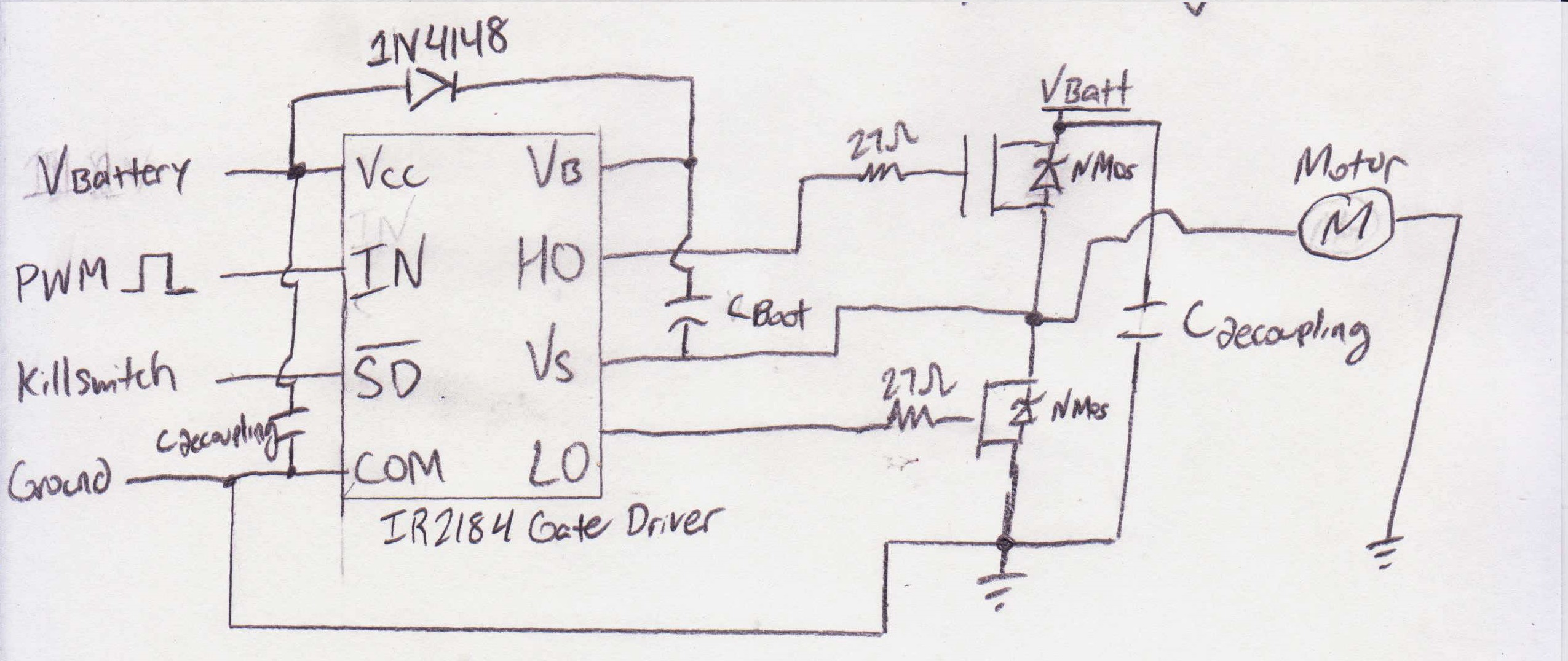
To implement the bootstrap capacitor and dead time, we utilized the IR2184 gate driver chip. From the datasheet, we saw that this chip had a relatively low switching time, had a high output voltage, and can output enough current to sink the NMOS gate capacitance. This chip would bias the high side and low side MOSFETs out of phase with each other and with added dead time. This would replace the BJTs in our initial circuit design and required only one PWM signal from the Arduino. Additionally, the IR2184 incorporated the circuitry to use bootstrap capacitors. To size this capacitor, we utilized an equation provided by the manufacturer. However, we found through experimentation that a 470 microfarad capacitor works well.

Line detection - Data Acquisition

For the competition, the official track would a line of white tape that is laid on the floor. Underneath the tape would be a wire carrying an alternating current. We had the option between using an optical sensor or an inductive sensor. The optical sensor would utilize the contrast between the tape and the floor. The inductive sensor would probably use wire coils and measure the induced current to detect the line. We opted for the optical sensor because it seemed easier to implement and test with.

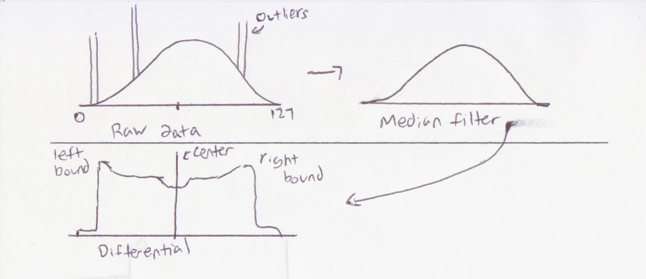
We used the Parallax TSL1401 Linescan camera. It is a one dimensional camera and has a resolution of 1 x 128 “pixels”, meaning that it only sees a horizontal line. Each “pixel” operates as a register for detected brightness intensity values. The register values range from 0 to 1023, where 0 corresponds to completely dark and 1023 corresponds to completely white. For each scan, the camera would take a snapshot of the floor and fill its registers with the corresponding brightness values. It would then clock out these 128 register values for the Arduino to analyze and then start another scan. The sensitivity of the camera’s sensor could be adjusted via clock timing so we could compensate for changes in external lighting.

Line detection - Data Analysis

From the camera data, we could infer that the high intensity values correspond to the white line, whereas the low values correspond to the dark carpet. However, the raw data from the 128 registers would show outliers or incorrect numbers. The camera sometimes reported high values even though the sensor lens was blocked for testing. To fix these error, we implemented a median filter with window size 5.

This filter took 5 values (eg: registers 5 to 9) and take the median of the set. This median would be appended to a new array. The “window” would be incremented by 1 (eg: registers 6 to 10) and the median would be taken from that set. This process repeated until all 128 registers were read and filtered. The final array was used for further analysis.

After median filtering, we differentiated each value with respect to its adjacent neighbor. For example, the value in array index 0 was subtracted from the value in array index 1. This difference was then appended into a new array. The next entry into this new array would be the difference between values in indexes 1 and 2. This process of subtracting adjacent numbers repeated for the remaining numbers.

From this differential array, we looked for the largest positive and negative value (maximum and minimum). The largest positive value indicated a transition from dark carpet into white tape. The largest negative value indicated a transition from white tape into dark carpet. The difference between the indexes of these two values would correspond to the middle of the white line. This “middle index” was then utilized for our proportional controller.

Proportional Controller and Servo Control

Our servo was used to steer the vehicle. When we seated our servo into the car chassis, we deduced the servo PWM values that correspond to the maximum steering range. A PWM value of 50 steered the front wheels to the far left direction. A PWM value of 115 steered to the far right. The median 55 shifted the wheels to move forward.

Experimentally, we found that the white line had a width of 40 pixels. The servo would lock to the far right or far left position when the middle index was close to the array edges. When the middle index was less than 20, the servo would lock to the far left. When the middle index was greater than 108, the servo would lock to the far right. This established our maximum boundaries for movement and computation.

For the car to follow the line, the middle index of the white line should ideally match with the middle index of the camera array. To accomplish this, we used a proportional gain controller that was modeled by the following equation.

Output = [(Kp * Error) + P_steadystate] * Tuning_value

Error: Difference between center index of the white line and the middle of the camera array Output: The PWM turning value for the servo was would reduce the error

P_steadystate: The output of the controller if where was no error. This corresponds to the value of 87, which maps the servo forward and makes the car move straight.

Kp: Proportional gain. The first component is the difference between the PWM values of the servo for far left and far right positions.The second component of proportional gain is the difference between the locking boundaries for the camera array. Proportional gain is the ratio between these

Tuning value: This initially had a value of 1 and was tweaked incrementally to fine tune car performance.

This proportional controller scheme aims to reduce the error to zero so that the camera tracks the center of the white line. The linescan camera was positioned so that it looks a couple inches ahead of the car. In one frame, the system would detect a curve, calculate the necessary PWM value to reduce error, and then map the servo accordingly. In the next frame, the linescan array would refresh and the process would repeat again.

Our system could be summed up as followed:

1. Linescan camera takes snapshot of line as a 128 pixel array.

2. Arduino performs median filtering to eliminate outliers.

3. Arduino detects the line and calculates its center index.

4. Proportional controller calculates PM value and turns the servo.

Conclusion

In the end, we managed to navigate most of the track. On the final curve at 10 feet from the finish line, our car swerved out of the track. Despite this, I think we did pretty well. Our current system only uses a proportional gain controller, meaning that the speed of the car is not factored into the equation. This is detrimental because the car speed is not constant despite running a constant PWM signal to the gate driver. The motor RPM is dependent on the voltage of the battery.

If we were to continue this project, we would add a rotary encoder in a feedback loop so that we can manage the speed of the car. Additionally, we would implement a Pure Pursuit controller schema, which adjusts the speed according to line curvature.